As we all know, sorting is the process of rearranging a sequence of objects to put them in some logical order. Today, almost all programming languages implement the Sort method in their official library. The programmer can invoke it with a compare logic, so it seems there is no longer any need to learn a sorting algorithm. But I want to say that when we build a huge system, the ability to process detail and design the structure are both important. In some scenarios, we need to develop the data structure and algorithm ourselves; only then can we improve the program’s performance and resolve significant problems.

Similarly, the experience of learning algorithms gives us essential knowledge to learn ideas from other large systems. So many problems have been perfectly solved in these large systems; if we want to gain power from these great projects, we need to understand their language. And the algorithm is a vital part of this kind of language.

There are many interesting sorting algorithms, and we don’t want to focus on the implementation detail since different programming languages have different syntax, and it will result in different codes. Spending too much time on the details like this is not what we want. So we’ll focus on specific topics and try to illustrate the mechanisms behind the algorithms. But I will paste the reference code at the end of the article, and you can run them yourself if needed.

Of course, talk is cheap, let’s start.

Overview of merge sort

The sorting algorithm we discuss in this section is based on a simple operation known as merging: combining two ordered arrays to make one large ordered array. Based on it, the algorithm is super simple. We divide a large array into two sub-arrays, sort the two halves recursively, and merge the result.

We can use a diagram to illustrate the procedure of this algorithm.

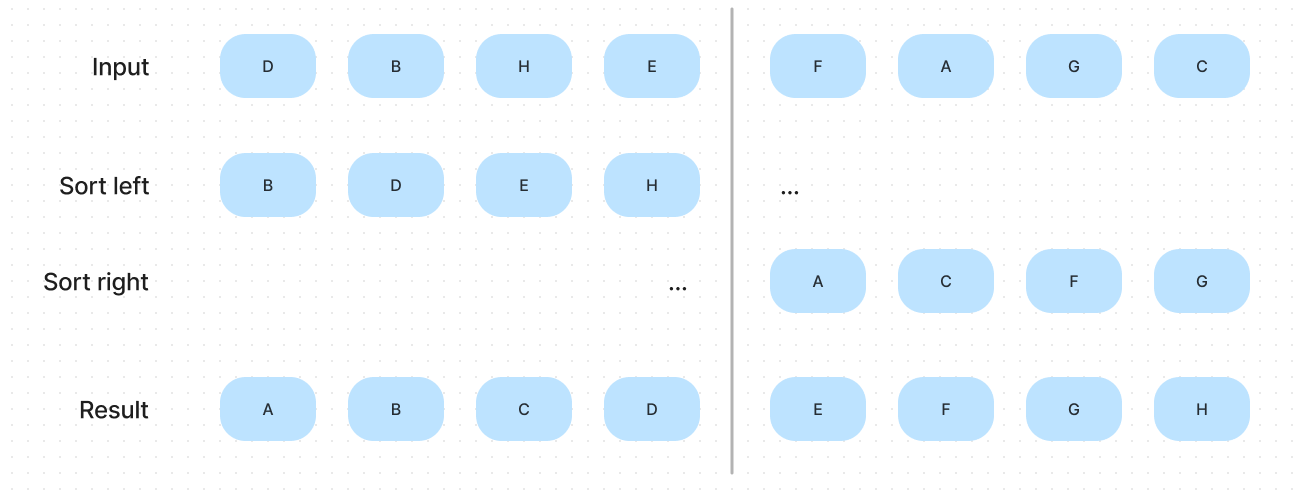
As shown in the illustration, if we have two sorted sub-arrays, we can merge them to get the sorted result. If you already understand this, please think, if each sub-arrays have three elements instead of the four shown in the illustration, is the procedure work? Of course, yes. Similarly, we can decrease the number of array elements until each sub-array has only one element. An array that has one element is a sorted array definitely.

That is the key to understanding this algorithm. We can find a way to divide the array until each sub-arrays have only one element and merge them. And the result of merging also is the sorted array, so we can keep merging until we get the final result.

This algorithm is one of the best-known examples of the utility of the divide-and-conquer paradigm of efficient algorithm design. In this kind of strategy, we solve a problem by dividing it into pieces, solving the sub-problems, then using the solutions for the pieces to solve the whole problem.

Merge

Let’s start with the merge procedure. The goal of this procedure is to merge two sorted arrays into one sorted array. Our idea is to declare two pointers, and each pointer starts at the beginning of two sub-arrays, traverse the array and compare each pair of a[i] and a[j], put the smaller item in the result array and move the pointer.

According to the analysis, it’s easy to write this method, and the following is the pseudo-code:

// lo: low bounds of the array
// hi: high bounds of the array
fun merge(array, lo, mid, hi):
  set i = lo
  set j = mid + 1
  set result = array

  for each position of the result:
    if left array is finished: copy right array into result .also { j++ }
    else if right array is finished: copy left array into result .also { i++ }
    else if a[i] < a[j]: copy a[i] into result .also { i++ }
    else: copy a[j] into result .also { j++ }

Improvement

As we can see, in the above method, we use extra array to store the original array. Since when we iterate over the array, some elements may be overwritten before being accessed. Declaring an additional array is a good solution but causes unnecessary memory waste. To address this problem, we can iterate the array from end to start.

Suppose we want to merge the nums1 and nums2, sorted in non-decreasing order. 0 is the placeholder.

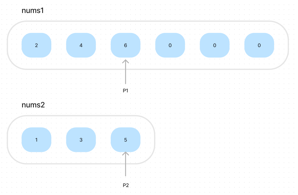
So the algorithm is easy. We iterate the nums1 from end to start, compare the current nums1[i] and nums2[j], put the lager one in the nums1.

// m - length of nums1, exclude 0
// n - length of nums2
fun merge(nums1, m, nums2, n):
  set i = m - 1
  set j = n - 1
  set k = m + n - 1   // end index of nums1, include 0

  while i, j is not out of scope at same time:
    if i is out of scope:
      set nums1[k] = nums2[j] .also { j-- }
    if j is out of scope:
      set nums1[k] = nums1[i] .also { i-- }
    else if nums1[i] > nums2[j]:
      set nums1[k] = nums1[i] .also { i-- }
    else:
      set nums1[k] = nums2[j] .also { j-- }
    k--

We can prove that at any time, no element will be overwritten before it is accessed. At any time, there are $m - (p_1 + 1)$ elements from nums1 are appended into the end of nums1, and $n - (p_2 + 1)$ elements from nums2 are appended into the end of nums1. On the right of the $p_1$, there are $m + n - (p_1 + 1)$ positions. We suppose at any time, the right of the $p_1$ have enough room to store sorted result:

It’s equivalent to

It’s always true. That means our assumption is valid. So we can say that when we use this algorithm to merge two sorted arrays, there aren’t elements being overwritten before access.

Top-down merge sort

The process of the top-down merge sort algorithm is dividing the array first util each sub-array has only one element, and merging them up to get the final result. The following is the pseudo-code:

// lo: low bounds of the array
// hi: high bounds of the array
fun topDownMergeSort(array, lo, mid, hi):
  // arrive at the leaf node of recursive tree
  if hi < lo: return
  set mid = mid index of the array

  topDownMergeSort(array, lo, mid)
  topDownMergeSort(array, mid+1, hi)
  merge(array, lo, mid, hi)

The recursion part is going to divide the original array into multiple sub-arrays. To truly understand this procedure, we must carefully analyze this recursive code’s behavior.

Procedures and the processes they generate

When we talk about the recursion, the most important thing is understanding the processes it generates. Otherwise, the recursion may be like a black box for us.

Linear recursion

Let’s start with factorial function, we have definition:

We can implement the following function to compute it:

fun factorial(n):
  if n = 1:
	return 1
  else:
    n * factorial(n - 1)  // unfold

When we invoke this function, the last line will unfold until it touch the bottom. The following diagram illustrate this process.

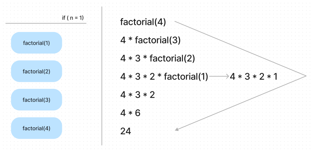
As the left part shows, the call stack will store the called function until the end condition is reached. At that time, the program will execute the function from top to down. If we consider the whole algorithm in terms of code execution, we can write the process at the right part.

We can easily observe that the whole process expands and contracts and the divider line is when the function reaches the end condition. So in other words, this procedure has 2 phases:

1. Expanding - store the function calling in the stack
2. Shrink - execute the functions from top to down

During the first step, the program record the function calls in the TODO list. And the order is very important, it will be reflected in the shrink phase. In addition to these, we need to notice these 2 properties of this algorithm:

1. The end condition will only be reached once
2. Once shrinking starts, no new function calls will be pushed onto the stack

Tree recursion

You might be curious, why do we talk about the linear recursion? That is because it helps us understand a widely used recursion form: tree recursion. It’s necessary to understand the top-down merge sort.

To illustrate the tree recursion, let’s consider the Fibonacci numbers. We can use the following formula to compute them.

According the formula, we can easily write out the code.

fun fib(n):
  if n = 0: return 0
  else if n = 1: return 1
  else: return fib(n - 1) * fib(n - 2)

According to our analysis above, the recursion means recording function calls in the TODO list. But the difference between this function and factorial is there are two recursion entries in the fib. This difference leads to 2 outcomes:

1. The end condition will be reached multiple times
2. During the shrinking phase, there may be other function calls pushed onto the stack

Which means the process of this function will be difference with factorial.

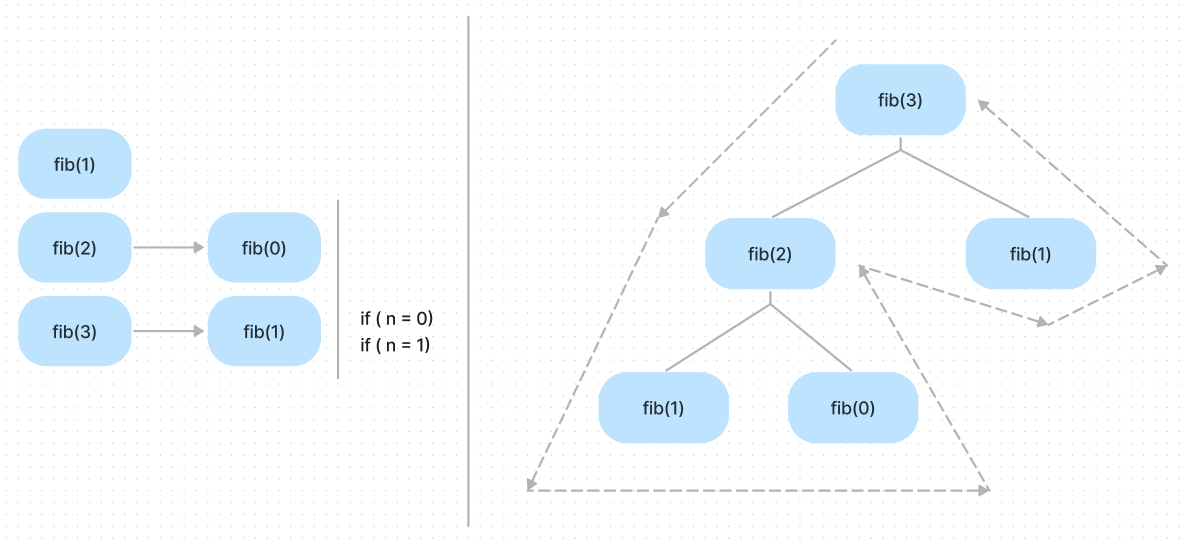
As we can see, the shape of the code execution is no longer a simple triangle, and it becomes a tree. Each function call that is pushed onto the stack can push new function calls onto the stack. It depends on whether the end conditions are reached or not.

The process of top-down merge sort

According the analysis above, we know if we want to understand a recursive algorithm, we need to know 2 things:

1. When the program reaches the end condition and how many times?
2. Which node will generate sub-tree?

Obviously, the end condition is the following code:

if hi < lo: return

If we observe the recursion code, we know as the function calls are pushed onto the stack, the original array will be divided into two same-length sub-arrays. This is because the end condition makes the current function call return when the sub-array only has one element. In other words, it’s the leaf nodes of the tree. It’s super easy to draw the process:

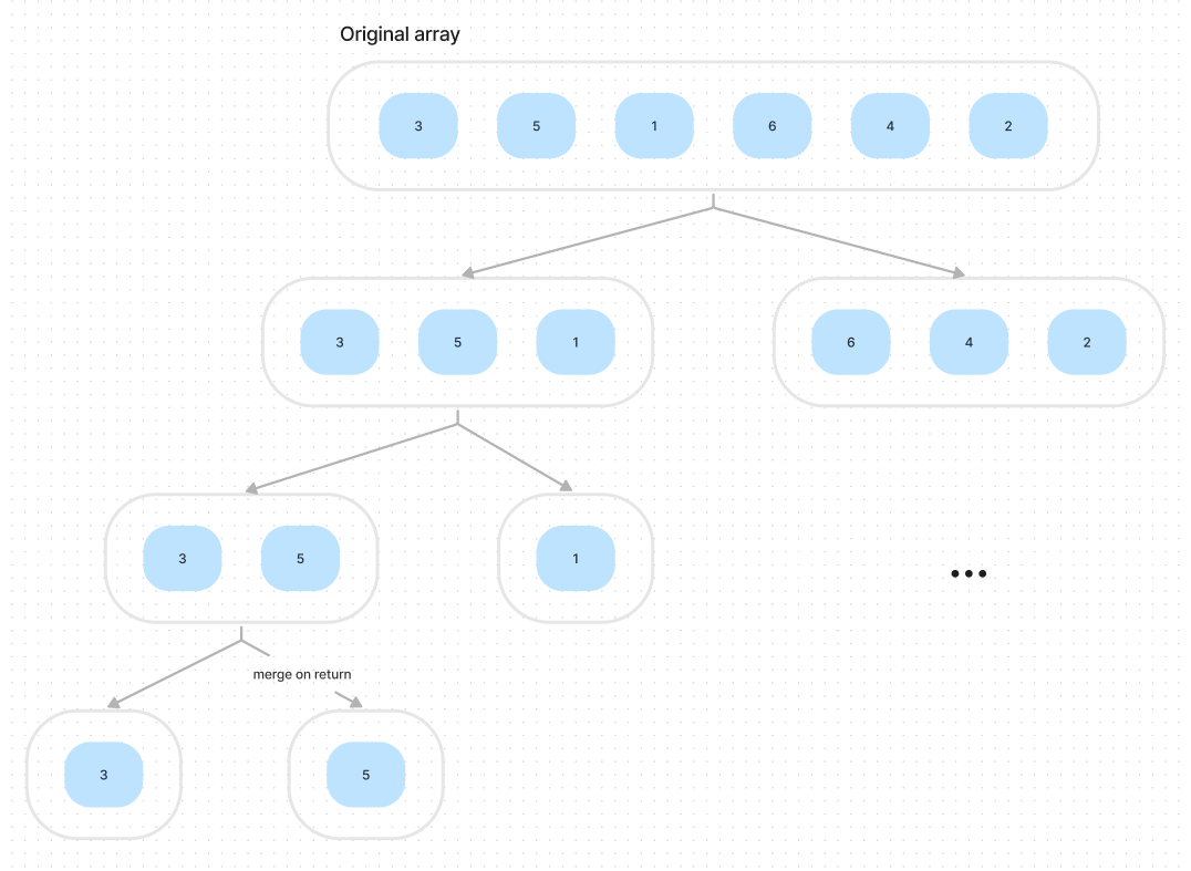
The program will try to divide the array as possible as it can, when it reach the end condition, which means the current array can’t continue to divide. If we observe the recursion code, we know this function is post order traversal.

topDownMergeSort(array, lo, mid)
topDownMergeSort(array, mid+1, hi)
merge(array, lo, mid, hi)

When the recursion stop and the major part start, the information of 2 sub-arrays can be accessed in the current environment, when I say information, I mean the elements of sub-arrays. So, for example, if the current environment is the [3, 5] array, the program knows the [3] and [5]. So the merge function will merge these two sub-arrays. And the result is [5, 3].

To be clear, although we use the word ‘sub-array’ to describe the results of recursive function calls, it doesn’t mean the algorithm creates two real sub-arrays. We only count the index of the original array. This tip can reduce a lot of useless execution.

Number of comparisons

Proposition: Top-down merge sort uses at most $N\lg{N}$ compares to sort any array of length $N$.

To understand this proposition, we can consider the diagram above. Each node depicts a merge, and the height of the tree h stand for the number of recursions.

For the $k$ th level, there are $2^k$ sub-arrays. Set the $h$ is the total levels of tree, the original array has $2^h$ elements, so for the $k$ th level, each sub-array has

elements. Thus each sub-array requires at most $2^{h-k}$ compares for the merge.

Thus we have $2^k * 2^{h-k} = 2^h$ total cost for each of the $h$ levels, we have $h$ levels, for a total of $h2^h$. Since $2^h = N$ and $h=\lg{N}$, so we have $h2^h=N\lg{N}$

Bottom-up merge sort

Another way to implement the merge sort is to process the whole array from bottom to top. We set a tiny number as the size of sub-arrays, pass those sub-arrays pairs to the merge function, increase the length by double it, and pass the new sub-arrays pairs to the merge function. Continuing until we do a merge that encompasses the whole array. The following is the pseudo-code:

// sz: size of sub array
// lo: lower bound of sub array
fun bottomUpMergeSort(array):
  for sz in 1..n, step sz:
    for lo in 0..(array.length-size), step sz:
      merge(
        array,  // the original array
        lo,     // start of sub array
        mid index of sub array,    // mid
        lower bound of next sub array or end of the array    // end of sub array
      )

When the array length is a power of 2, top-down and bottom-up merge sort perform precisely the same compare and array accesses, just in a different order. When the array length is not a power of 2, the sequence of compares and array accesses for the two algorithms will differ.

To proof this, we can print the size of sub-array when we use the merge sort. Here we have a exercise:

Q. Give the sequence of sub-array sizes after each merge performed by both the top-down and the bottom-up merge sort algorithms, for n = 39.

A. Since the top-down is tree traverse algorithm, so the size will effect each node of the recursion tree. The bottom-up merge is just iteration, which means the size will be stable for each iteration.

• Top-down merge sort: 2, 3, 2, 5, 2, 3, 2, 5, 10, 2, 3, 2, 5, 2, 3, 2, 5, 10, 20, 2, 3, 2, 5, 2, 3, 2, 5, 10, 2, 3, 2, 5, 2, 2, 4, 9, 19, 39.
• Bottom-up merge sort: 2, 2, 2, 2, 2, 2, 2, 2, 2, 2, 2, 2, 2, 2, 2, 2, 2, 2, 2, 4, 4, 4, 4, 4, 4, 4, 4, 4, 3, 8, 8, 8, 8, 7, 16, 16, 32, 39.

The complexity of compare-based sorting algorithm

Proposition: Compare-based sorting algorithm need at least $lg{N!} \sim Nlg{N}$ to sort a array with $N$ items.

To prove this, we can consider the following comparison tree. An internal node i : j corresponds to a compare operation between a[i] and a[j]. The left sub-tree corresponds the a[i] is smaller than a[j], and the right sub-tree corresponds the a[i] is lager than a[j]. The leaf nodes mean a permutation. And it’s easy to know that a path from root to leaf corresponds to the sequence of compares that the algorithm uses to establish the ordering in the leaf.

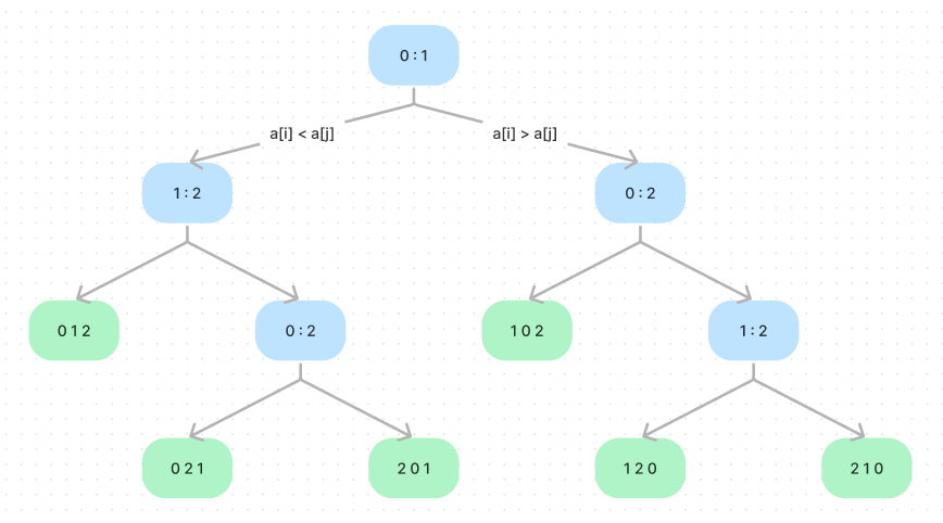
It’s easy to know for an array with $N$ items, there are $N!$ different permutations, which means the compare tree has $N!$ leaves at least. If there are fewer than $N!$ leaves, some permutations are missing from the tree. The longest path from the root to leaf is critical since it measures the worst-case number of comparisons used by the algorithm.

If we fill all these internal nodes and leaf nodes, the compare tree will become a complete binary tree. For a complete binary tree of height $h$, it has at most $2^h$ leaves. According to the analysis in this section, we have:

The height path $h$ corresponds to the worst-case path; in other words, $h$ is the worst-case number of compares. To get the scope of $h$, we take the logarithm (base 2) of both sides of this equation.

We will know the number of comparisons used by any compare-based algorithm must be at least $lg{N!}$. Apply Stirling’s approximation; we have $lg{N!} \sim N\lg{N}$.

Sample code

You can get code for this algorithm on GitHub.

Reference

• SICP, 1.2 Procedures and the Processes They Generate
• Algorithms 4th, 2.2 mergesort